Filtering is an important part of observational seismology because the amplitude of different seismic waves depends on a number of factors such as earthquake size, source-to-station distance (and geometry), etc. and the amplitude of the Earth's background motions also vary from place to place and over time. Both also depend on the frequency of the observation, so finding the "right" bandwidth to insure optimal signal-to-noise ratios in the data generally dictates some filtering is necessary.
I can't explain filters and time-series analysis in a simple online document, you have to track down the background elsewhere. What I want to do in this document is simply show you how to examine SAC's filters using SAC's impulse function generator.

Generating an Impulse Signal
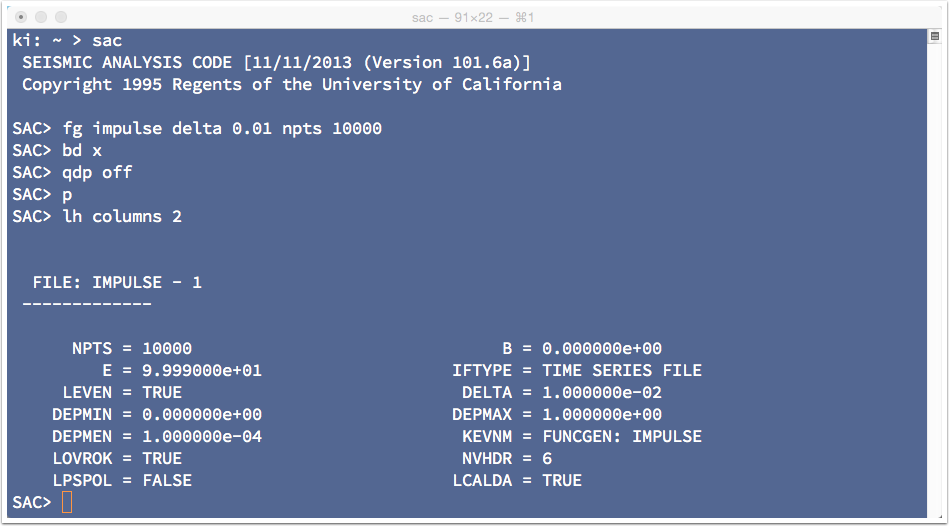
We are going to examine filter impulse responses and transfer functions using SAC. Obviously the first step is generating an impulse. We'll use SAC's funcgen command, which I abbreviate as fg. The next screen shot shows the command to do so (fg impulse delta 0.01 npts 10000), which generates an impulse with a sample interval of 0.01 s that's 100 seconds long.
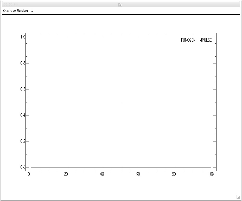
Here's the plot of the impulse
We can scale the signal using the div (or mul) commands.
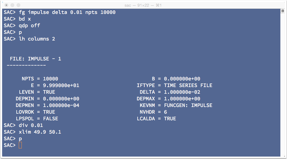
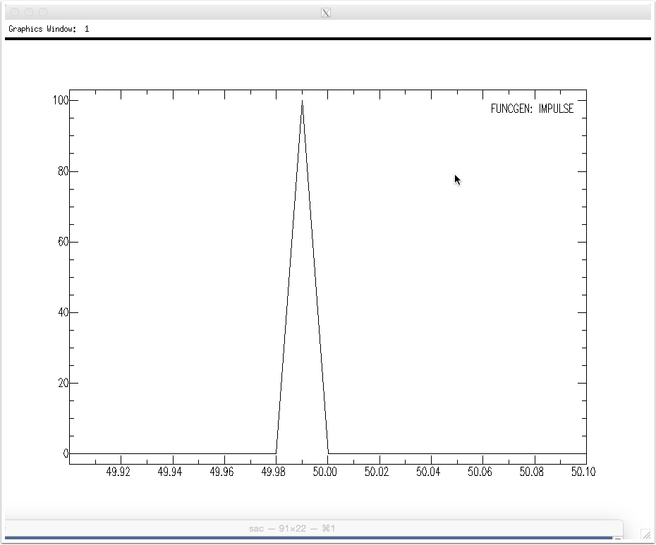
Here's a closeup of the impulse. Note that because we sample the signal, the impulse is really more like a triangle than a true impulse. Also, SAC by default generates a unit-amplitude impulse. For spectral work, we want a unit-area impulse. If we divide the impulse by the sample interval, dt, the triangular signal will have unit area. If you integrate the function you will obtain a maximum value of unity.
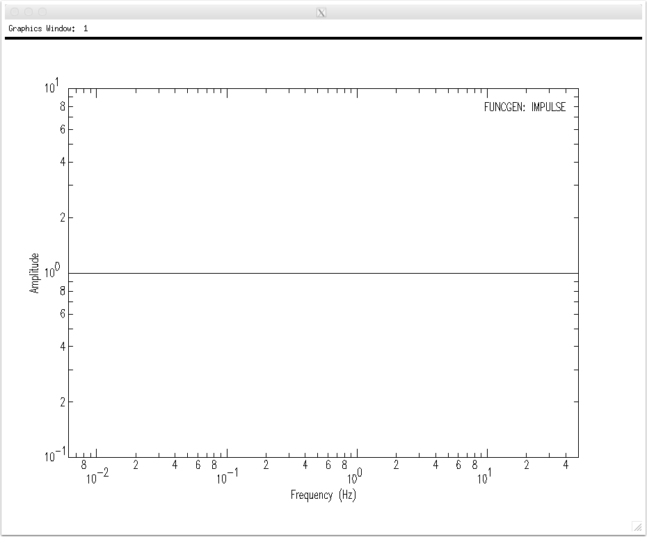
This isn't a perfect impulse (it's a very narrow triangle), but the spectrum is flat in our bandwidth. We can compute and plot the spectral amplitudes using the fft command.
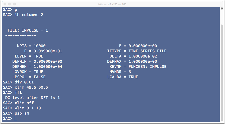
The Nyquist frequency for our signal, which is controlled by the sample rate, is 1/(2*dt), which is 50 Hz.
Butterworth Filters
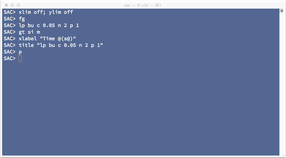
SAC has a number of filters, we'll only examine a few, you can explore the others on your own. Let's low-pass filter the signal to emphasize frequencies below 0.05 Hz (20 seconds period). I also increased the plot font size, added an xlabel, and included the filter command in the plot using the title command.
Exploring SAC's Filters
The filter command (lp) includes options
lp- low-pass filterbu- set the filter subtype to Butterworthc- set the corner of the filter to be at 0.05 Hzn- is the number of poles in the Butterworth formula (controls filter sharpness)p- number of filter passes (1 or 2 passes); one pass for a causal filter, two for a zero-phase, acausal filter.
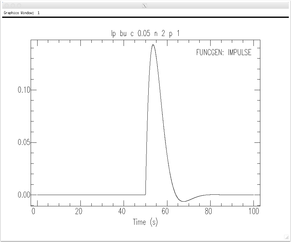
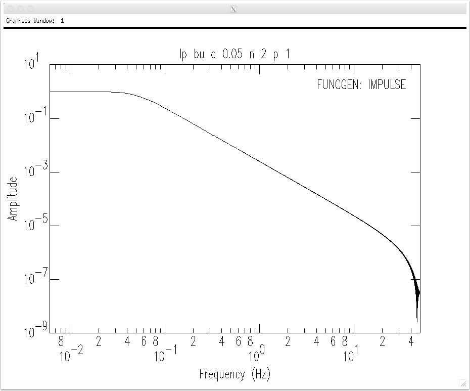
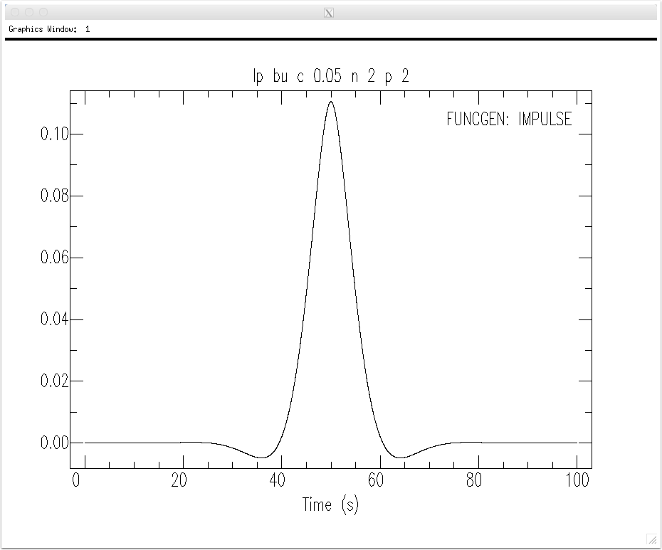
The filter's impulse response is shown below.
The transfer function is the spectrum of the impulse response. The transfer-function amplitude spectrum is shown below. Note that for frequencies lower than the filter's corner frequency, the response is generally flat and equal to unity (that's why it is a low-pass filter).
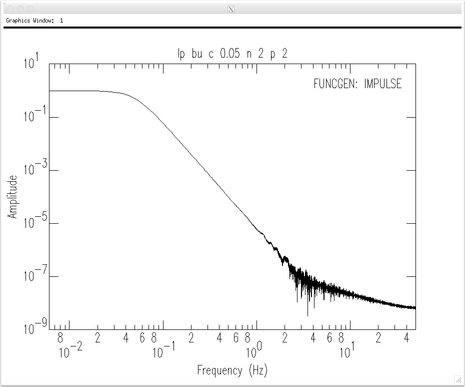
By repeatedly using the fg command you can explore the character of the filter for different options. For example, a two-pass filter looks like this.
And it's spectrum falls off more quickly than the one-pass filter because the filter is applied twice. Note that we enter the realm of numerical noise just above one Hz in this example.
Explore
You can examine filters using SAC and explore many of the fundamental concepts of elementary time-series analysis using SAC and the relatively simple functions that the funcgen command can generate. I encourage you to do so, you will become more comfortable with SAC and you really should understand the responses of any filters that you use on your data during result.