Seminar in Seismic Tomography Instructor: Charles J. Ammon Exercise 02

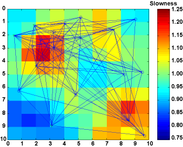
A Two-Dimensional Tomography Laboratory Objective: To study a simple two-dimensional travel time tomography problem using MATLAB. Although only 80 observations are used in the inversion, the geoemtry and coverage problems in the example are selected to mimic common problems encountered in research. The model dimensions are 10 x 10 (100 unknowns). Procedure: You should complete the following calculations and numerical experiments using MATLAB. The files that you need are in ~ammon/MLTomo. A script called tomo2d.m will allow you to import the ray paths and the travel times for the model. It also has some options for plotting the model, computing a solution, and showing the ray paths. You should study the script to become familiar with MATLAB. The problem that you will solve (and the solution) is shown in the following figure. Study the path distribution and write a paragraph commenting on what parts of the model will have good, fair, and no resolution and why. The solution and the paths:   To get started, type tomo2d('init') and MATLAB will ask you to find the pathmatrix file (thePaths) and the observations file (theObs). Select those files. Once you have selected those files you need to set some variables to be global variables (accessible from scripts and the MATLAB command line). Execute the following: global L; global obs; global t; global pls; global nobs; global nr; global nc; global shat; global soln; global coverage; Then do a 'whos' to see what variables are available.

Use MATLAB to complete the following calculations. Submit a write-up of your work that summarizes the calculations and includes key figures - an implicit requirement for each exercise is that you intelligently describe the results and the implications of each experiments. Put special emphasis on comparing various measured of resolution - ray path plots, coverage, resolution matrices, spike tests, checkerboard tests. Be concise but thorough, I will not accept excessively long submissions. Any submission that contains only MATLAB output and undocumented diagrams will not be accepted.

A)	Solve the tomography problem using the "generalized inverse approach" described in Aki, Christofferson, and Husbeye (1977). You should look at Jackson (1972) to see more explicit details on how to compute the inverse operator using the singular value decomposition of L. Use the "pinv" command in MATLAB to help you perform the truncation analysis.
B)	Solve the same problem using the stochastic, or damped least-squares method also described in Aki, Christofferson, and Husbeye (1977). Try a range of damping factors and make a tradeoff between damping model length and match to the observations. Recommend a preferred model based on this curve. Compute the resolution matrix for the damped least-squares approach. Plot the rows of the resolution matrix corresponding to a cells located at the third column and third row and at the sixth row and eighth column as a two-dimensional images (the slowness model is stored in row-major order beginning with the upper left of the image).
C)	Add 5% of random noise to the travel times and part A and choose a preferred model. Show the trade-off curve between truncation fraction, or damping value and model length (insure that your range in fit to the observations makes sense in light of the level of noise you added to the signals).
D)	Check the resolution using "spike tests" with a 10% spike located in the third column and third row from the upper left of the image. Perform another spike test for the cell in the sixth row and eighth column from the upper left. For the cell Construct the "target" model Set the slowness of the cell to 1.05 Set the slowness of the other cells to 1.00 Compute the travel times through the target model (t = L s) Invert these travel times for an estimate of s. end loop over cells Plot the results of the spike tests using the imagesc command. Which cell is better constrained? How does the spike-test information compare with the resolution matrix information regarding these same cells?
E)	Compute and plot the coverage matrix corresponding to the paths stored in the matrix L.
F)	Create a model with blocks 2 x 2 of alternating slownesses of 0.95 and 1.05. This will help: % % compute the checkerboard model % c = 0.95*ones(10,10); skip=1; for i = 2:2:10, if(skip == 1) for j = 1:4:9, c(i-1,j)=1.05; c(i, j)=1.05; c(i-1,j+1)=1.05; c(i, j+1)=1.05; end else for j = 3:4:9, c(i-1,j)=1.05; c(i, j)=1.05; c(i-1,j+1)=1.05; c(i, j+1)=1.05; end end skip = skip * -1; end % check it with a plot imagesc(c) % % store the model in a vector called cs % k = 1; for i=1:10, for j=1:10, cs(k) = c(i,j); k = k + 1; end end Create a set of observations using the supplied ray paths and invert this checkerboard model. Plot the result and comment on the reconstruction fidelity (does it recover the pattern, the amplitudes, etc.).