The Elastic Rebound Conceptual Model For Earthquakes

Supplemental Notes for GEOSC 488 - Charles J. Ammon / Penn State

Contents

Introduction

Reid (1910) developed the elastic rebound model of earthquake recurrence using geodetic observations from the 1906 San Francisco Earthquake. The idea is conceptually valuable in that it captures the relationship between strain accumulation (now known to result from plate motions) and eartquake occurrence. A similar idea had been espoused by G. K. Gilbert a few decades earlier, but Reid (1910) had more quantitative information to be more specific than Gilbert. While the model is conceptually pleasing, it has little predictive value for specific faults because of complexities in fault and near-fault structure, and because of fault interactions.

Conceptual Models

Keep in mind that these models are conceptual. They explore some of the simplest possible variations that may operate during earthquake cycles. Most fault systems are more complicated because of variations in fault strength with position and perhaps time (as a result of variations in lithology, fluid processes, etc.) and because most faults are part of larger fault systems and faults interact. Still, these models are valuable tools to describe the patterns associated with faulting.

Stress and Coseismic Slip

The elastic rebound model is generally illustrated in introductory courses using a deforming fence, road, or similar marker. At this level we can begin to think of the model in terms a fault held locked together by friction between earthquakes, The strength of the fault, S, is the stress (force per unit area) that the deformed rocks adjacent to the fault must exert on the fault to overcome the friction holding the rocks together at the fault.

When the earthquake occurs, the stress drops and the two sides of the fault are offset. The amount of offset varies, but generally larger earthquakes have larger coseismic slips. In the following computations, we will illustrate the relationship between the stress on the fault and time, and coseismic slip and time. We adopt a simple linear relationship between stress drop and slip - this is part of the conceptual model, but with real earthquakes the relationship is not quite so simple, earthquake stress drops usually range betwee 0.3 and 10 MPa, with an average value near 3 MPa. The value does not correlate strongly with earthquake magnitude, suggesting that earthquake stress drops are roughly constant. A good value to keep in mind is 3 MPa. For the computations below I use values for the maximum and minimum stress values of 10 MPa and 2 MPa, simply so that you can see the patterns more clearly. The stress drops are thus less than 6 MPa.

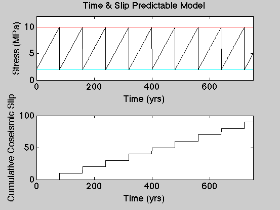
Time and Slip Predictable Model

The simplest "recurrence" model of earthquakes is a sequence of repeating events that relieve the same stress in each event. If the strain assumulation rate (plate motions) is constant then the time between earthquakes will be the same as will the slip in each event. For these simple computations, I put in some numbers for the stresses and the slip values, but while these are typical stress drops and slip values in earthquakes, the relationship is artificial and only useful in a conceptual way.

% Simple Elastic Rebound model
t = 0:1:750; % time of the cycles in years
Smax = 10;
Smin = 2;
% use the remainder function to make a saw-tooth function
tau = Smin + rem(0.1*t,(Smax-Smin));
dSlip = 10;
dTau = 0.1;
%
clf;
subplot(2,1,1);
% plot two bounding lines for the min and max stress
%   and the stress as a function of time.
plot([t(1);t(length(t))], [Smax; Smax],'r-', ...
    [t(1);t(length(t))], [Smin; Smin],'c-', ...
    t,tau,'k-');
xlabel('Time (yrs)','Fontsize',18);
ylabel('Stress (MPa)','Fontsize',18);
set(gca,'Fontsize',18);
title('Time & Slip Predictable Model');
xlim([0 750]);
ylim([0 12]);
%
% compute the slip from the stress asumming a constant
%  slip in each event (dSlip).
slip(1) = 0;
for i=2:length(tau)
    if(tau(i) - tau(i-1) < 0)
        slip(i) = slip(i-1) + dSlip;
    else
        slip(i) = slip(i-1);
    end
end
subplot(2,1,2);
plot(t,slip,'k-');
xlabel('Time (yrs)','Fontsize',18);
ylabel('Cumulative Coseismic Slip','Fontsize',18);
set(gca,'Fontsize',18);
xlim([0 750]);

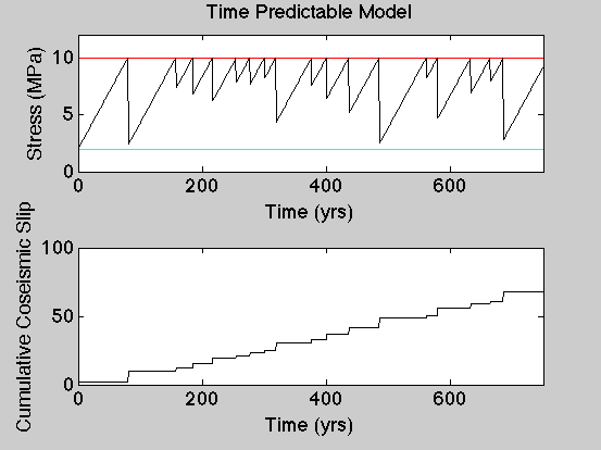
Time Predictable Model

In the time predictable model, the strength of the fault is constant and earthquakes only occur when that failure stress is breached. Thus if we know the load on the fault at any time during the cycle, and we know the stress increase rate, we can predict when the next earthquake will occur.

t = 0:1:750; % time of the cycles in years
% compute the stress as a function of time,
%  the failure stress has a random component.
tau(1) = Smin;
for i=2:length(tau)
    tau(i) = tau(i-1) + dTau;
    if(tau(i)>= Smax)
        tau(i) = Smax - (Smax-Smin) * (1 - rand);
    end
end
dSlip = 10;
%
clf;
subplot(2,1,1);
% plot two bounding lines for the min and max stress
%   and the stress as a function of time.
plot([t(1);t(length(t))], [Smax; Smax],'r-', ...
    [t(1);t(length(t))], [Smin; Smin],'c-', ...
    t,tau,'k-');
xlabel('Time (yrs)','Fontsize',18);
ylabel('Stress (MPa)','Fontsize',18);
set(gca,'Fontsize',18);
title('Time Predictable Model');
xlim([0 750]);
ylim([0 12]);
% Compute the coseismic slip as a function of time.
% The coseismic slip for each event is proportional to
%  the amount of stress drop.
slip(1) = Smin;
for i=2:length(tau)
    if(tau(i) - tau(i-1) < 0)
        slip(i) = slip(i-1) + dSlip*(tau(i-1)-tau(i))/Smax;
    else
        slip(i) = slip(i-1);
    end
end
subplot(2,1,2);
plot(t,slip,'k-');
xlabel('Time (yrs)','Fontsize',18);
ylabel('Cumulative Coseismic Slip','Fontsize',18);
set(gca,'Fontsize',18);
xlim([0 750]);

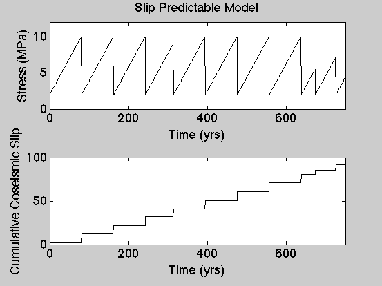
Slip Predictable Model

In the slip predictable model, the strength of the fault is varies - earthquakes occur at different levels of stress on the fault. Thus if we know the load on the fault at any time during the cycle, and we know the stress increase rate, we can predict the stress level at any time which we can use to predict the size of an earthquake if it were to occur at any particular time.

% Simple Elastic Rebound model
tau(1) = Smin;
for i=2:length(tau)
    tau(i) = tau(i-1) + dTau;
    if(tau(i) >= Smin + (Smax-Smin)*rand*75)
        tau(i) = Smin;
    end
    %
    if(tau(i) >= Smax)
        tau(i) = Smin;
    end
end
%
clf;
subplot(2,1,1);
% plot two bounding lines for the min and max stress
%   and the stress as a function of time.
plot([t(1);t(length(t))], [Smax; Smax],'r-', ...
    [t(1);t(length(t))], [Smin; Smin],'c-', ...
    t,tau,'k-');
xlabel('Time (yrs)','Fontsize',18);
ylabel('Stress (MPa)','Fontsize',18);
set(gca,'Fontsize',18);
title('Slip Predictable Model');
xlim([0 750]);
ylim([0 12]);
% Compute the coseismic slip as a function of time.
% The coseismic slip for each event is proportional to
%  the amount of stress drop.
slip(1) = Smin;
for i=2:length(tau)
    if(tau(i) - tau(i-1) < 0)
        slip(i) = slip(i-1) + dSlip*(tau(i-1)-Smin)/(Smax-Smin);
    else
        slip(i) = slip(i-1);
    end
end
subplot(2,1,2);
plot(t,slip,'k-');
xlabel('Time (yrs)','Fontsize',18);
ylabel('Cumulative Coseismic Slip','Fontsize',18);
set(gca,'Fontsize',18);
xlim([0 750]);

Published with MATLAB® 7.4