Western United States Structure
For details, please see our paper in Geophysical Research Letters.
Chengping Chai, Charles J. Ammon, Monica Maceira, Robert B. Herrmann (2015), Inverting Interpolated Receiver Functions with Surface‐Wave Dispersion and Gravity: Application to the western US and adjacent Canada and Mexico, Geophysical Research Letters, 42(11), 4359–4366, doi:10.1002/2015GL063733.
The velocity model is also available at the IRIS Earth Model Collaboration (Link).
Receiver Function Interpolation/Smoothing
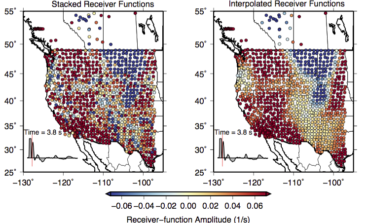
Receiver functions have been widely used to estimate the depth and velocity contrasts for major vertical structure boundaries. However, scattering effects and noise contaminate the receiver function observations. Receiver functions are normally averaged (stacked) at a single station to supress noise. Due to the limited receiver function waveforms available for temporary stations, single station average may not reduce noises significantly. We developed a receiver function interpolation/smoothing technique to supress the scattering effects and noise using waveforms from adjacent stations. In the following figure, we compared the stacked (single station averaged) receiver functions with our interpolated/smoothed receiver functions at time 3.8 s (after direct P wave arrival time). Each dot represents a seismic station. The colors show the receiver function amplitudes. At 3.8 s, the converted phase from Moho is already arrived for red regions, while the Ps phase is still coming for yellow regions. The blue colors indicate negative amplitudes, which are mainly caused by shallow sediments. The difference indicates the crust is thinner for red regions (since Ps phases arrive earlier than 3.8 s) while thicker for the yellow regions (Ps phases arrive later than 3.8 s). Comparing the stacked receiver functions with the interpolated ones, we found that first order features from the stacked receiver functions were extracted out through interpolation/smoothing. The scattering effects were reduced though the interpolation process. The first order features are visiable in the stacked receiver functions, but more consistent for the interpolated receiver functions.
Download an Animation:
Simultaneous Inversion
Known by researchers for decades, geophysical inversions are usually non-unique, which means more than one model can explain observations. Constraining the subsurface structure with only one type of observations usually leads to large uncertainty. Combing independent observations can help to alleviate the nonuniqueness and reduce the uncertianty. We incoporated interpolated receiver functions, Rayleigh-wave group velocities and gravity observations to better constrain the subsurface seismic structure. Receiver functions are sensitive to the velocity contrast, and Rayleigh-wave dispersions constrain the smoothed absolute velocity values. Gravity observations were filtered to provide additional constraints at shallow depth. Emperical density/shear-velocity relationship was used to relate gravity observations with shear velocities. Integral of these three geophysical data sets allow us to construct a reliable estimate of subsurface structure. Our interpolated receiver functions have a similar lateral sampling distance as the surface-wave dispersion. We found the interpolated receiver functions are more suitable for joint inversion of receiver functions and surface-wave dispersions.
Shear Velocity Structure
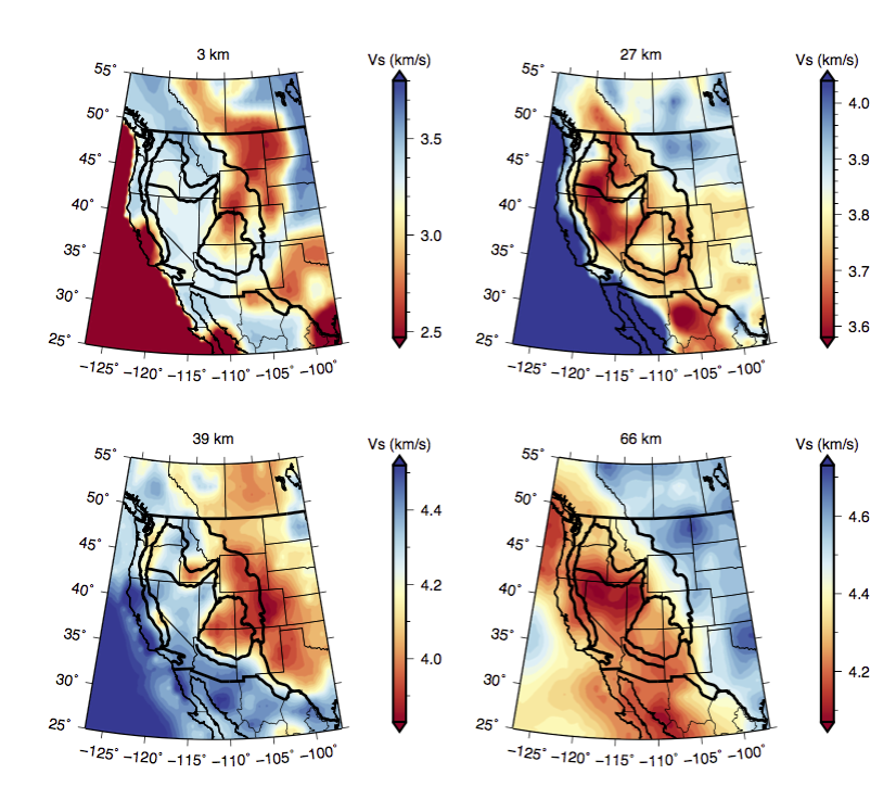
Our shear velocity model agrees with published models to the first order. As shown in the following figure, major basins shown slow speeds at 3 km depth. At 27 km depth, the shear velocity is faster beneath the craton region and slower beneath the Basin and Range region. At 39 km depth, shear velocity for blue colors is close to tipical mantle speed, which indicates the Basin and Range region has thin crust. On the other hand, the interior part of continent has a thicker crust. At 66 km depth, we see a well defined boundary between the western part and eastern part of the region.
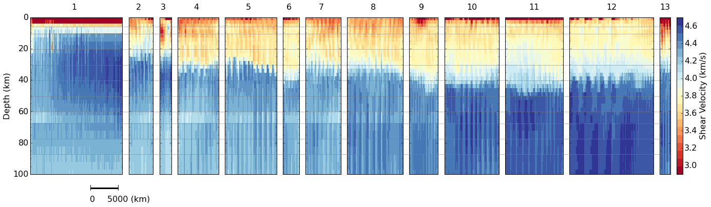
We also used cluster anlaysis to explore our 3D model. Similar 1D velocity profiles are group together in the cluster analysis. We found the spacial distribution of the clusters correlates with the geological provinces. Cross section for each cluster is shown in the follwoing figure. The number at the top is refferred to a geological region. Within each region, the cross section is plotted from left to right and from top to bottom (like reading a book). We can see the crust is getting thicker as we move to the east. And the upper mantle velocity is increasing from west to east on land.
Download
The velocity models and related codes can be downloaded through the following links.