Receiver-Function Inversion


Important Note on Amplitude Convention: The inversion codes use a normalized Gaussian filter that will affect the amplitude of the receiver function. If you use your own deconvolution program, you must alter the amplitudes so that the Gaussian filter has unit time-domain amplitude (not unit area). See the inversion code for details of the normalization.

Background and Details

There are three programs that are used to invert receiver functions: snglinv, smthinv, and manyinv. All the codes execute a linearized, iterative inversion of a specified waveform. They incorporate a minimum roughness constraint to remove non uniqueness problems from each individual inversion - but the full nonlinear problem of finding acceptable models is not unique.

Partial derivatives are calculated using a finite-difference approximation, but the computational demands have been reduced greatly by George Randall's algorithm based on the intricacies of Kennett's (1983) reflection-matrix approach to seismogram computation.

Langston pointed out the sensitivity of the structure to shear waves, and Tom Owens demonstrated that the shear-wave partial derivatives are much larger than the compressional wave partial derivatives, so the inversion is formulated to estimate the shear-velocity.

At the present, a default Poisson's ratio of 0.25 is assumed in the inversion, but plans are to allow a more flexible inversion in the near future (as soon as I find time). The change will not affect how the program is run, it will simply adopt the Poisson's ratio of the input model.

The inversions also use the "Jumping" algorithm which was developed by R. Parker and allows a solution for a velocity model at each iteration as opposed to a solution for a velocity-model correction vector. Thus minimum roughness constraints are applied directly to the velocity model, not the correction vector.

Let m represent the velocity model, dm a velocity correction vector, d the residual vector, and G the matrix whose i'th column is the partial derivative of the receiver function with respect to the shear velocity in layer "i". The initial model is called mo and the model we seek is called m, where m = mo+ dm. Then we can invert either of two equations with very little computational difference. If we want to solve for the model correction vector, we can solve:

G dm = d

Or, we can modify that equation algebraically by adding Gmo to both sides

G dm + G mo = d + Gmo

And using the fact that m = mo + dm, we can construct another equation which we can invert directly for the model, m.

Gm = d + Gmo

Inverting the first equation above for the correction vector, dm, is called creeping, inverting the third equation directly for m is called jumping.

We use a singular-value decomposition to compute the matrix inverse and solve the inverse problem. However, because we add smoothness constraints, we do not need to truncate the singular values and thus the resolution matrix is an identity matrix. This of course is a meaningless quantity in this case, we have in essence changed the original inverse problem to one where we are seeking the smoothest solution in the vicinity of the initial model that fits the data.

The inclusion of smoothing constraints also limits the utility of standard least-squares inversion uncertainty analysis. Since we have added the smoothness constraints as a priori "data", the estimated variance of the model parameters depends on the smoothness constraints. If you greatly increase the importance of the smoothness constraints, the model-parameter uncertainties will decrease, but that's not a reflection of high-quality observations, it's a reflection of your faith in the smoothness constraints.

A Typical Modeling "Schedule"

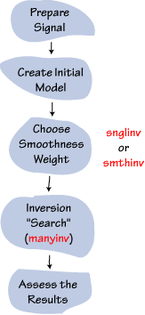
A general flow chart of the inversion procedure is shown to the right. The procedure consists of preparing the observations, constructing an initial model, choosing a smoothness weight parameter, inverting the waveforms and assessing the significance of features in the results. The inversion is really a a search for models fitting the observations using a gradient-based inversion algorithm to map out local minima.

Preparing the Observations

First, you have to get your data ready. Check to see that you don't over sample the observations, usually a sample rate of about 10 samples per second is suitable (delta = 0.1) for studying first-order crustal features. When we were computing the deconvolutions, we used a 20-30 second time shift in the pulse so that we could get a clear idea of the processing noise in the resulting deconvolution. That long signal "leader" is not useful in the inversion, so usually, we cut the signal about 5 seconds in front of the first peak before beginning the inversion.

In general, you should cut the observations such that later arrivals, which may not be generated by the first-order structure of the region are excluded. However, if you make the time series too short, you might have to "zero-pad" the end of the signal.

You can use SAC to insert zeros at the beginning or end of any record. First you issue the "cuterr fill" command, then set a cut window wider than the signal. As you read in the waveform, SAC will fill the signal with zeros out to the window specified by the cut command.
r a_rcvr_ftn.eqr
rmean
taper
w over
cuterr fill
cut b +0 e +20
r
w over
cut off
 

The above commands will add 20 seconds onto the end of the trace (e is the trace end time, e +20 sets the cut to 20 seconds later than e). The "rmean" command may be overkill since the equalization should produce a zero-mean result (the mean of both components was removed before the deconvolution). The taper command is important to insure that no sharp ofsets are introduced when you add zeros to the ends of the trace.
Preparing an Initial Model

To get started, you can use either a model that you have chosen from your own forward modeling, or from another study of the region you are working on, or from a region with a similar geologic history. Usually, we use rather thin (2-2.5 km) layers throughout the model which provides some freedom in where precisely the larger velocity contrasts will occur. If you know the shallow structure very well, you could add finer detail in that region where the wavelengths are most likely minimum. Use the program icmod to create a model if you have not already done so.

Inversion Overview

The overall inversion procedure includes three different inversion steps. First, a single inversion of the waveform is performed to estimate the number of iterations required for convergence. Then a suite of inversions with a varying roughness requirement is performed to estimate the value of the roughness weight to use in the "final" inversions. For these inversion, we use the number of iterations determined from the first run. Finally, the initial model dependence is explored using the number of iterations obtained in the first inversion, and the smoothness weight obtained in the second set of inversions. Each of these steps utilizes a different inversion program.

Initial Inversion - Estimating the number of iterations required

The number of iterations in any inversion depends on the complexity of the structure and the closeness of the initial model to a structure that matches the observations. To invert one single waveform for one velocity model, you use the program "snglinv". Here is a shell script for snglinv:

snglinv > test.log <<
initial_model
5
0.1
01
0.001
n
1
target.eqr
0.06
5.
2.5
end
#
# initial model
# maximum # of iterations per inversion
# smoothness trade-off parameter
# inversion ID #
# SVD truncation fraction
# Include a high-pass filter?
#   if yes it will ask for the corner next
#    then it will ask for the number of filter passes (1 or 2)
# # waveforms
# sac file name(s)
# horizontal slowness (ray parameter (s/km))
# waveform delay (cut rftn to have a few seconds in front)
# Gaussian width factor (same as data)
 

The comments at the bottom explain the input parameters, and in this case we are inverting a waveform called, "target.eqr" using an initial model called "initial_model". The run includes 5 iterations and uses a smoothness weight of 0.1 ( a pretty-good value to start; if you have a "low-frequency" receiver function, say from a Gaussian width factor of 1.5 or less, try a smoothness value of 0.5). A small truncation fraction is included just in case some near-zero singular value escapes through the minimum roughness constraint. The inversion "ID" is used in the file names.

The output is saved in the file "test.log" and within an ASCII velocity model (in TJO format) from each iteration and the predicted receiver function corresponding to each of the inversion models. The file "wvfrm01" contains the waveform that was inverted (which could be different than that input if you applied the high-pass filter). When you compare the results, you should compare the syn01.01?? files with wvfrm01. The last integer in the file name of the model and the synthetic seismograms refers to the iteration numbers. Here is a listing of the directory ... RInversion/Test.Snglinv

Makefile        inv.mdl.0102    svalues_inv01   syn01.0104      wvfrm01
README          inv.mdl.0103    syn01.0100      syn01.0105
initial_model   inv.mdl.0104    syn01.0101      target.eqr
inv.mdl.0100    inv.mdl.0105    syn01.0102      target_model
inv.mdl.0101    run_test*       syn01.0103      test.log
 

You look at the results and see at which iteration the waveform is mostly matched (quantitative misfits are in the log file, if you want to be specific, but usually, a visual match is more appropriate). Once you have decided on the minimum number of iterations that it took to converge, you are ready to search for the smoothest model that matches the observations. (If you want to be conservative, add a few iterations to the number; it won't take too much more time).

Here's a SAC macro to step through the results of an inversion (it will prompt you for the inversion number):

The SAC Macro

Comments

xlim 0 35
qdp 1200
fileid t n
color on inc on list r b
 
r wvfrm01
sqr
int
setbb spwr &1,depmax
 
do file wild syn01.010??
 
r wvfrm01
subf $file
sqr
int
setbb misfit &1,depmax
 
evaluate to c0 %misfit / %spwr
evaluate to c1 100 * %c0
evaluate to pmis 100 - %c1
 
title '(CONC 'This Model Fits ' 
    ' ( BEFORE '.' ' %pmis ' ) ' 
    ' percent of the signal power.' )'
 
r wvfrm01 $file
ch b 0
p2
 
pause
 
enddo
Some plot
initializations
 
 
Read in the waveform,
compute & store its
power in the blackboard
variable "spwr".
 
 
Now, loop (using
filename  wild cards) 
over each iteration &
compute the misfit
power & store in
"misfit".
 
 
Next compute the
percent misfit
of the signal.
 
Build a plot title
containing the misfit.


Read in the waveforms
and plot them.


End of the loop.

Finding the smoothest model

To find the smoothest model, you simply vary the smoothing weight parameter using the program "smthinv". The preparation is the same as for "snglinv", but the input is slightly different. For this program, you enter a minimum and maximum value for the smoothness weight, and then you again examine the results visually, choosing the smoothness weight value that produces the smoothest model that still fits the observations relatively well.

smthinv > test.log <<
initial_model
3
0.0
1.0
0.001
n
1
target.eqr
0.06
5.
2.5
end
#
# initial model
# maximum # of iterations per inversion
# minimum smoothness trade-off parameter
# maximum smoothness trade-off parameter
# SVD truncation fraction
#   if yes it will ask for the corner next
# # waveforms
# # waveforms
# sac file name(s)
# slowness
# waveform delay
# Gaussian width factor (use same as data)
 

The output files are similar to those from "snglinv" except now the inversion number is updated in the name of the models and the predictions. The last two numbers are still the iteration number, the fourth and third from last identify the inversion number. The singular values of the SVD are output in the svalues_inv?? files so that you can see the effects of the smoothness on the inversion singular values. They are stored in SAC files (you can read them in and use "P2" to compare them).

To make a plot of the misfit versus the minimum roughness weight, you can extract the misfit values from the log file (assuming that you created the log file as it was in the above script). Again, look at the results and choose the smoothest model that fits the data to the level that you decide is appropriate.

Exploring Initial Model Dependence

Armed with the number of iterations necessary for a typical inversion to converge on a solution, and an appropriate value for the smoothing weight, you are ready to investigate the initial model dependence using the program "manyinv". In that program, an input model is perturbed and an inversion is executed. You can specify the number of inversion to perform and control the amount of perturbations to the initial model.

The initial-model perturbation scheme

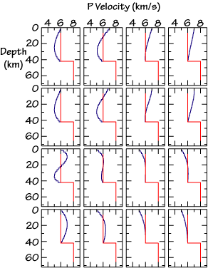
To perturb the initial model, a composite of a cubic perturbation and a random perturbation are added onto the layer velocities. The cubic perturbation is defined to apply broad changes to the initial model, such as raising or lowering the upper, middle and lower crust velocities. One of the three roots of the polynomial is systematically moved to different depths in the model - specifically there are four points for this root throughout the model. The specific location is not important, but that is the reason that the number of inversions completed by "manyinv" is a multiple of four.

An example of 16 model perturbations to a simple single-layer crust are shown to the right. The red line identifies the initial model, the blues lines, the perturbations. The first two rows are similar, but not exact. The cubic perturbation scheme is not ideal but does shift the initial model using broad changes.

The random perturbations can be used to add short wavenumber fluctuations to a model.

Included below is an example script for running the test inversion with manyinv.

manyinv > test.log <<
input_model
0.75
7.8
20.
4
0.1
2
0.01
n
1
target.eqr
0.06
5.
2.5
end
#
# initial model
# maximum cubic perturbation
# stop perturbing at this velocity
# maximum random perturbation (in % of cubic perturbation)
# number of iterations per inversion
# smoothness trade-off parameter
# number of inversions (x 4) 6 => 24 inversions
# singular value truncation fraction
# high-pass filter the waveforms (y or n)
#   if(yes)
#       Enter fmin
#       Enter npasses (1 or 2)
# number of waveforms
# sac file name(s)
# horizontal slowness (ray parameter)
# waveform delay
# Gaussian width factor
#
 

One problem with manyinv is that it creates a lot of files. Not all the files fit the observations so the first thing to do is sort those that fit from those that don't. I use SAC and a visual inspection to assess the quality of the fit. The quantitative estimates of the misfit are included in the program output (which if you directed into a log file, has been saved). Here's a little macro to help you quickly peruse the fits. You may want to keep track of which results fit acceptably. You will be prompted for the iteration number (use a value like "05", not "5".

The SAC Macro

Comments

xlim 0 35
qdp 1200
fileid t n
color on inc on list r b
 
r wvfrm01
sqr
int
setbb spwr &1,depmax
 
do file wild syn01.??$iter
 
r wvfrm01
subf $file
sqr
int
setbb misfit &1,depmax
 
evaluate to c0 %misfit / %spwr
evaluate to c1 100 * %c0
evaluate to pmis 100 - %c1
 
title '(CONC 'This Model Fits '
  ' ( BEFORE '.' ' %pmis ' ) '
  ' percent of the signal power.' )'
 
r wvfrm01 $file
ch b 0
p2
 
pause
 
enddo
Some plot
initializations
 
 
Read in the waveform,
compute & store its
power in the blackboard
variable "spwr".
 
 
Now, loop (using
filename  wild cards) 
over each iteration &
compute the misfit
power & store in
"misfit".
 
 
Next compute the
percent misfit
of the signal.
 
Build a plot title
containing the misfit.
 
 
Read in the waveforms
and plot them.


End of the loop.

Overview | Data Prep | Source Equalization | Creating a Model
Computing the Response | Inverting a Waveform | References
Back to Ammon's Home

Prepared: June/July/August 1997 - Charles J. Ammon, Saint Louis University