Creating a Velocity Model

TJO Model Format

The receiver function programs use an ASCII velocity model format designed by Tom Owens. You can edit the file using an ascii editor or you can use the program "icmod" (which abbreviates "interactive creation of models" (?)). The first line in the file contains the number of layers and a comment (the comment may be copied into the SAC header of synthetic seismogram, depends on the seismogram calculation code you use).

The format has spaces for Vp, Vs, density, thickness, four attenuation values, strike, dip, and Poisson's ratio. Vp and Vs are in km/s and density is in g/cm^3, the strike and dip are in decimal degrees. The attenuation values are not used in the standard synthetic seismogram programs and so are usually left as zeros. Likewise, the value of Poisson's ratio is completely determined by Vp and Vs, and so it is not really used. Here is a sample velocity model:

  3 testmod                         
  1   5.5700  3.2158  2.5524 15.0000  0.0000  0.0000  0.0000  0.0000  0.2500
  2   6.7500  3.8971  2.9300 15.0000  0.0000  0.0000  0.0000  0.0000  0.2500
  3   8.2000  4.7343  3.3940  0.0000  0.0000  0.0000  0.0000  0.0000  0.2500

Program icmod

The program icmod gives you a range of options for inputting the velocity structure, too many in fact. Here's an example execution of the program.

your options are:
   1 -- input all parameters for each layer
   2 -- same as 1 except default qp,qs,strk,dip
   3 -- input pv & poissons ratio; same defaults as 2
   4 -- input sv & poissons ratio; same defaults as 2
   5 -- same as 3 except default rho and poissons rat
   6 -- same as 4 except default rho and poissons rat
 please input option no. 
5
 choose between:
   1 -- inputting layer thkness, or
   2 -- depth to bottom of layer.
1
 choose between:
   1 -- tjo output format
   2 -- srt output format, or
   3 -- output in both formats.
1
 input is in free format, type 0.0 for h/z to end input
 lyr
 vp  h/z
   1
6,10
   2
6.2,10
   3
6.3,10
   4
6.4,10
   5
8.0,0.
 lyr    vp      vs      rho     h/z     qp      qs      strk   dip     por
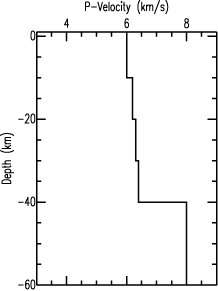
  1   6.0000  3.4641  2.6900 10.0000  0.0000  0.0000  0.0000  0.0000  0.2500
  2   6.2000  3.5796  2.7540 10.0000  0.0000  0.0000  0.0000  0.0000  0.2500
  3   6.3000  3.6373  2.7860 10.0000  0.0000  0.0000  0.0000  0.0000  0.2500
  4   6.4000  3.6950  2.8180 10.0000  0.0000  0.0000  0.0000  0.0000  0.2500
  5   8.0000  4.6188  3.3300  0.0000  0.0000  0.0000  0.0000  0.0000  0.2500
are these ok?  y
split lyrs for inv? n (this doesn't do anything)
output file name?   the_file_name
title?    my_title
 

Note that you enter a layer thickness of zero to terminate the input loop. To quickly enter just Vp and layer thickenss, start the program input off with: a 5-enter, 1-enter, 1-enter (where -enter indicates hitting the return key). That will create a model with a standard Poisson's ratio of 0.25.

Plotting A Velocity Model

To view the velocity model, use the program vplot[s] to create a SAC file.

Here is a sample of a program run of vplot[s]. (I call it vplots because some UNIX machines have another command vplot, and I want to avoid confusion (the source code is really vplot.f)).

vplots
velocity file  the_file_name
List the site model? (y or n) y
 file: junk       model:  thetitle     5 layers 
 
 
 lyr     vp      vs     rho      h     qp      qs     strike    dip
   1     6.00    3.46    2.69   10.00    0.00    0.00    0.00    0.00
   2     6.20    3.58    2.75   10.00    0.00    0.00    0.00    0.00
   3     6.30    3.64    2.79   10.00    0.00    0.00    0.00    0.00
   4     6.40    3.69    2.82   10.00    0.00    0.00    0.00    0.00
   5     8.00    4.62    3.33    0.00    0.00    0.00    0.00    0.00
 

The program vplot[s] outputs three unevenly spaced SAC files: the_file_name.vp, the_file_name.vs, the_file_name.rho. You can plot the model in SAC. For example, try this: