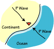
The basic idea governing receiver-function data organization is to group the signals into "clusters" that sample the same structure. Most observations are also naturally clustered by the distance and azimuth of appropriate sources.

Waves approaching a seismometer from different directions may sample very different structures. An extreme example is shown to the right.

At most stations, the structure varies with azimuth and even in the simplest cases, the response can vary with distance from the station.

We usually group the observations by azimuth, then distance. We stack, or average, waveforms from the same azimuth and distance range, although at times, when the coverage is very broad, studying the response as a more continuous function of azimuth or distance is a nice way to study the structure.

Click here for a data-organization "flow" chart.

For the Rftn analysis, you need three-component observations, preferably with a wide bandwidth. If the instrument response of the components is matched, you do not have to remove the instrument effects before proceeding, but you must insure that the gains are equalized before proceeding to the receiver function deconvolution. To correct for differences in instrument gain, use the scalar division command "div" in SAC. If the instruments are not matched, you should remove or replace them with a set of uniform instrument responses, which you can do with the "transfer" command in SAC.

For example, suppose I had three seismograms from SNZO: myevent.z myevent.n myevent.e The instrument responses for the station are matched, with the exception of a small variation in the gain. To remove the slight difference, I would execute the following SAC commands:

     r myevent.e myevent.n myevent.z
     div 6.465442 6.478608 6.307450
     w over
 

The gains are actually the values above x 10^13, but the constant factor doesn't matter, only the variable coefficient.

Once you have the instrument response worked out, you next need to supply the information necessary for SAC to rotate the horizontal seismograms into the theoretically based radial and tangential directions. Specifically, you set several header variables in each of your waveforms:

• The event latitude and longitude
• The component azimuth
• The component incident angle

To set these values for each seismogram, you use the change header command:

The "r" command reads the seismogram into memory. The "wh" command writes the header, saving the appropriate information. Once this information is stored in the header, SAC will automatically compute the distance and back azimuth of the observation. Latitude is positive north of the equator, longitude is positive east of Greenwich, England. Enter the numbers in decimal degrees. The cmpaz is the component azimuth also in decimal degrees, north is 0°, east is 90 °, etc. After you have made these additions to the file header values, you can view the great-circle distance and back azimuth using the "lh" command

      lh gcarc baz
 

Windowing the Data

The final data-preparation stage consists of windowing the P waveform from the pre-signal noise and the rest of the seismic signal. The amount of record that you use depends somewhat on the seismogram. You want to isolate the P-waveform from the remaining signal. For the usual teleseismic distances (30° to 95°) you are usually safe by using about 60 seconds of signal "leader" and 60 seconds of signal following the onset of the P wave. The precise duration can vary if needed, these are typical values. At times details in the estimated receiver function may be sensitive to substantial (10s of seconds) variations in length, and you can get a feel for the variations by comparing several lengths of signal during the source equalization procedure.

To cut the desired part of the seismogram from SAC, you use the "cut" command. The SAC time reference system is based on two different times. A reference time which is stored in the header "kzdate and kztime" and the begin time of the trace. For our purposes, the begin time is most important, since we will use that value to reference the cut. Suppose that the P-wave onset occurs at about 80 seconds into the seismogram, then we would want to window the signal between 20 and 140 seconds. We also should remove the mean and taper the ends of the signal to avoid signal processing artifacts later in the processing. The following SAC commands with perform the desired operations.

     r  myseismogram.e myseismogram.n myseismogram.z
     qdp  off
     p1
     cut 20 140
     r
     rmean
     taper w 0.1
     w over
 

Once the data are windowed, we are ready to calculate the the radial and tangential receiver functions. See the Source Equalization Page for a discussion of the procedure.

A SAC Macro For Pre-Processing Raw Observations

If you have many waveforms to prepare, the above will get tiring. Here is a SAC macro that I have used to handle cutting, detrending, tapering, and separating noisy observations from the better signals. The data are stored in files named: *BHZ, *BHN, *BHE, where the * means "whatever". Make a directory with a copy of your observations (Data files will be overwritten if you execute this macro - work with a copy of the data!) and execute this macro.

The macro is interactive - you will be picking the approximate P onset from the vertical component using the PPK command in SAC. When the cursor appears, place it at the P-onset time and enter "t" "0" (that's a zero) to set the t0 header value. Enter "q" to go onto the next part of the macro, where you decide whether to keep the data or move them into the "Noisy" directory. You only need to identify the time the time within a few seconds, don't agonize over precision.

If the data are all noisy, just enter "q" and then enter an "t" later to move the signal to the "Trash" directory.

The mean and a trend are removed from the observations and a cosine taper is applied on the left and right fifth (about 25 seconds if you keep the time limits in the macro) of the signal.

You must edit the "div" line to put in the correct instrument gains, or just delete that line and correct the gains later.

sc mkdir Trash
sc mkdir GoodOnes
qdp off
ygrid on
do file wild *BHZ
 setbb vert $file
 setbb east '( CHANGE 'BHZ' 'BHE' %vert )'
 setbb north '( CHANGE 'BHZ' 'BHN' %vert )'
 r %vert %east %north
 synch
 w over
 r %vert
 rmean
 rtr
 ppk
 setbb t0 &1,t0
 r %vert %east %north
 ch t0 %t0
 w over
 cut t0 -60 t0 +90
 r %vert %east %north
 rmean
 rtr
 taper w 0.2
 div 6.307450 6.465442 6.478608
 w over
 p1
 setbb resp (REPLY "Enter t to trash the file")
 if %resp eq "t" then
   sc mv %vert Trash
   sc mv %east Trash
   sc mv %north Trash
 else
   sc mv %vert GoodOnes
   sc mv %east GoodOnes
   sc mv %north GoodOnes
 
 endif
 cut off
enddo

Make directories.
 
 
 
Key on the
vertical...
 
Synchronize the 
file start times.
 
 
Pick the P onset &
mark it in the
header.
 
Cut the data 60 s
before and 90 s 
after the P onset.
 
 
Remove the mean, a
trend, and correct
the gain of each
instrument.
 
 
 
Move the files into
the directory
"GoodOnes" if they
look useable, or
into "Trash" if 
they look really
bad.
 
 
 
Turn cut off and do
the next one.