Each seismogram is a composite of source (rupture kinematics, etc.) and propagation effects (depth phases, etc). For receiver function studies, we must isolate the near-receiver structure from the source and distant structure effects.

The availability of three-component observations allows us to use the redundant source information on the three components to "equalize" source and near-source structure effects and isolate the receiver structure effects on the waveforms.

Langston (1979) developed the source equalization procedure remove the effects of near-source structure and source time functions. The procedure works quite well and enables the use of shallow earthquake waveforms in receiver structure studies.

The earliest receiver function studies such as Phinney (1964) worked in the frequency domain using the ratio of amplitude spectra to estimate the gross characteristics of structure. Langston (1979) extended the method to include phase information by using a complex frequency-domain ratio and inverse transforming back into the time domain. For his deconvolution he used a water-level stabilization method and a low-pass Gaussian filter to remove high-frequency noise not filtered by the water-level.

Frequency-Domain Deconvolution (Ideal Case)

Let w represent angular frequency (2*pi*f), Z(w) and R(w) represent the Fourier transforms of the vertical, radial components of motion, and E_R(w) the Fourier transform of the radial receiver function. The receiver function is defined by

$E\_R(w)\; =R(w)\; Z*(w)/Z(w)Z*(w)$

Z*(w) represents the complex conjugate of Z(w). A similar equation can be written for the tangential component of motion, defining the tangential receiver function.

To simplify the result, Langston (1979) introduced a low-pass Gaussian filter, G(w) into the procedure. The Gaussian was chosen because of its simple shape, zero phase distortion, and lack of side-lobes.

$E\_R(w)\; =[R(w)\; Z*(w)/Z(w)Z*(w)]G(w)$

While the above equation is the definition of a receiver function, it cannot be used to compute observed seismograms because small or zero values of Z(w)Z*(w) cause numerical problems in the calculation. There are several approaches to avoid this problem, the simplest is the ad hoc approach called water-level deconvolution. This was the approach adopted by Langston (1979) and is still a very good method when the data quality is good. Other approaches such as time-domain inversion of the algebraic convolution equations are available, but in each instance a parameter similar to the water-level parameter must be selected (damping value, truncation fraction, etc.).

Water-level Deconvolution - (Non-Ideal Case)

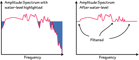
In water-level deconvolution, the way we avoid division by small numbers is to replace small values in the denominator with a fraction of the maximum value (for all frequencies) value of the denominator. The fraction is called the water-level parameter (the water-level is the fraction multiplied by the maximum denominator amplitude), and is chosen by trial and error. The consequence of replacing small values with larger values in the denominator is an attenuation of frequencies for which the vertical component has a small amplitude. At times the water-level can act as a high-pass, low-pass, and notch filter.

The appropriate water-level fraction is controlled by the the signal-to-noise ratio and nature of the vertical component seismogram and is chosen by examining the results of several trial water-level fractions and choosing the lowest water-level that produces acceptable noise levels in the corresponding receiver function.

The smaller the value that you can use the better, since the water-level filter can cause distortions of the receiver function. Typical values to investigate are 0.0001, 0.001, 0.01, and 0.1, but don't be afraid to explore other values.

Usually the value is chosen by studying the effects on the radial component and the same value is used for the tangential receiver function (since the same denominator is used in each case).

How to Judge Source Equalization Results

If you are going to estimate the water-level fraction using trial and error, you must be able to judge the results. Since you don' know the answer before hand, this can be tricky. There are several clues to assessing the deconvolution stability: How high is the pre-signal noise? How consistent are the results from different, but similarly located earthquake waveforms? Is the result temporally localized?

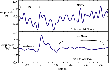
As discussed below, the deconvolution program requests a phase shift for the result. The phase shift moves the start of the receiver function from zero (the beginning of the time series) to the value you input. If you have "padded" the seismograms with noise or zeros before the deconvolution, you can shift the signal 30 seconds or so, and thus have a segment of the receiver function that under ideal circumstances should be zero. That part of the trace can be used to assess the level of processing noise in the receiver function.

Two extreme examples are shown below, the Gaussian filter removed most of the higher frequencies from these receiver functions, and the result should be simple. The top trace is very noisy because the original signals were not very strong and the ambient seismic noise was relatively high. Note the high, pre-signal noise at the beginning of the trace, and how the noise runs through the entire length of signal shown. Most crustal receiver functions finish their reverberations within 20-40 seconds after the first arrival (exceptions exist and are indicative of strong near-surface heterogeneity). The bottom panel is a plot of a very stable deconvolution. The pre-signal noise is low, and the signal is concentrated in the first 20 seconds following the P arrival. The acausal trough in front of the P-wave is caused by the limited bandwidth of the signal. When comparing this observation with model responses, it would be wise to band-pass filter both to a common bandwidth (that is, you can introduce a similar acausal trough into the model responses).

Note that the units of a receiver function are 1/time - the physical units of the seismograms are canceled in the spectral division, but the transformation back into the time domain brings in an extra factor of df, which has units of 1/time. Often, the responses are shown without units, so I wouldn't worry about this detail.

The Gaussian Filter

The low-pass Gaussian filter commonly used to "clean up" high-frequency noise in the receiver functions is

G(w) = exp(-w^2 / (4 a^2))

The frequency content is controlled by the Gaussian filter-width parameter, a. The filter gain at w = 0 is unity (a unit-area pulse). The Fourier transform of a Gaussian is a Gaussian, so the filter is gentle. If we decide to quantify the filter by the frequency at which it has a value of 0.1, we can construct the following table:

An easier way to remember these values is to note that the values approximately follow the rule of thumb: the filter gain is 0.1 at a frequency approximately equal to a/2 . In the time domain, the width of the Gaussian pulse is about 5/[3*sqrt(a)] (this is the full-width at half the maximum).

The Averaging Function

To see the effects of the water-level parameter on the resolution of the source equalization procedure, we compute what is called the averaging function. The averaging function is calculated by deconvolving the vertical component of motion from itself, using the chosen water-level parameter. If the water-level fraction is zero, the result is a perfect Gaussian (from the low-pass filter included in the procedure. Large water-level values produce a broadened, and often distorted averaging function. For receiver function analyses, a water-level value of 1.0 produces a scaled version of the cross-correlation of the horizontal and vertical seismograms rather than the desired deconvolution.

This view of the averaging function is valid assuming that there is neither noise nor uncertainty in the underlying assumptions in the deconvolution. Now this is obviously not the case with observed seismograms, but the averaging function remains a good way to see the effects of the water-level on the waveform and can provide a guide to what details in the resulting receiver function that you should not interpret.

Program pwaveqn

The program that is used to perform the source equalization is called pwaveqn. The "n" at the end identifies the normalization procedure where the averaging function is scaled to unit amplitude. pwaveqn works with either synthetic seismograms or real data, and will perform the rotation of observed north and east components into the radial and tangential directions. The program reads and writes SAC files and the IO parameters (filename, water level, Gaussian width factor, etc., see below) are entered interactively.

Here is a script that accepts command-line arguments and runs the pwaveqn:

#/bin/csh
#
# The files should be named:
#    basename[n,e,z]
#     and the event and station coordinates should
#     be in the header of the files.
#
if ($#argv == 0) then
 echo "Usage: equalize basename waterlevel gauss_width tshift"
 exit 1
endif
#
# Set up the input
#
set filename = $1
set outfile = $1
set waterlevel = $2
set gaussian = $3
set time_shift = $4
#
# Run the Program
#
pwaveqn << echo
$filename
y
n
$outfile
$waterlevel
$gaussian
$time_shift
n
echo
# All Done

Program Output

The output of the run would be SAC files named:

Iterative Deconvolution Notes

The iterative deconvolution code can be misused if you don't use it correctly. Use lots of bumps and let the iterative process run for a substantial amount of time. The specific number of bumps depends on the length of the receiver function and the Gaussian width. If you see "flat" regions in your receiever functions, make sure that you haven't undersampled the response by using too few "bumps".

The misfit between the observed radial seismogram and the receiver function estimate convolved with the observed vertical component is a valuable parameter to identify problematic deconvolutions. I usually stick to signals better than 90% fit but when data are hard to come by, I'll use 80%. Much of those impressive fits come from the P-wave, which is interesting, but not all that interesting. This is my preference, not a rigid rule - you should understand and analyze your own data to the point where you can make your own decision.

Amplitude Adjustments for iterdecon receiver functions

The iterative deconvolution scaling is different than that used in the waterlevel and the inversion codes (this is because I use the iterative deconvolution for source analyses, and the amplitude scaling is more important). The difference is really a convention - the ampltiudes in the receiver functions are used in an absolute sense (as they should be). Back when instruments were narrow band, we found that normalizing helped with some aspects of our analyses. This is not the case anymore, but the convention remains. Thus if you compute a receiver function with the iterative codes, but want to use them in the inversion codes, then you must normalize them by the area of the averaging function.